
NewVersion 1.0
Resistive Forces & Terminal Velocity
Drop a coffee filter, a steel ball, a raindrop or a skydiver and watch drag grow until it balances the weight, then compare linear and quadratic drag and fit the drag law to falling filters.
About this simulation
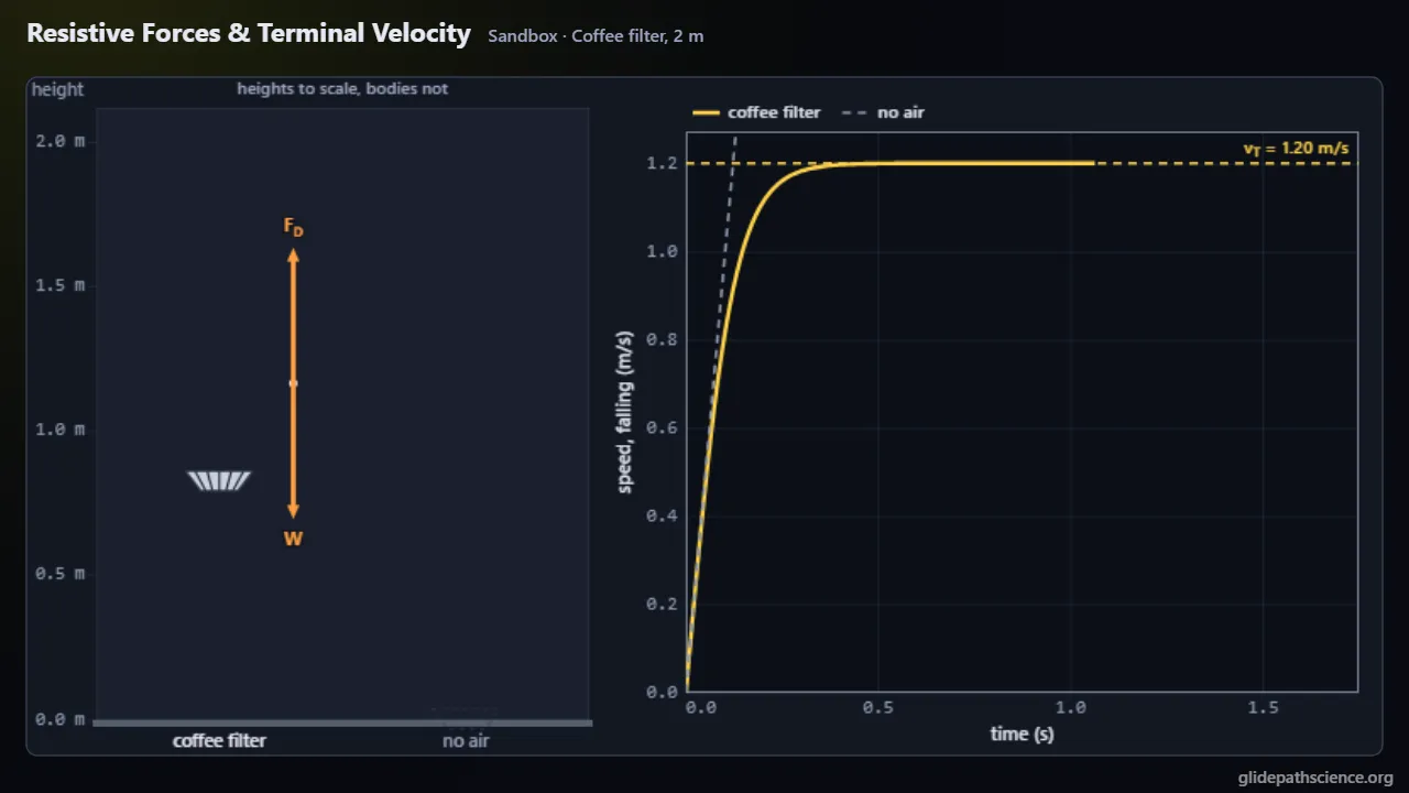
Why does a coffee filter drift down while a steel ball drops? Students release a body in air, water or glycerin, set its mass, area, drag coefficient, height and launch speed, choose the linear law, the quadratic law or none, add buoyancy, and read speed, height and acceleration graphs beside a no-air ghost and the other law, while the Reynolds number says which fits. A guided walkthrough at two levels runs from a ball and a filter dropped together through the forces on the way down, drag equal to weight, the terminal-speed formula, the speed–time graph, the parachute, fall times, raindrops and hail; the Advanced track adds linear drag solved exactly, its time constant, the tanh solution, the Reynolds number, an upward throw, the power at terminal speed and thin air. A Skydiver jumps from up to 6 km and opens a canopy; Coffee Filters drops stacks under a motion detector with honest noise and fits the drag law’s exponent. A concept challenge with Match the graph, and a prediction lab with Race to the ground, round it out.
What you'll learn
- Explain that a falling body speeds up until the drag, which grows with its speed, balances its weight; then the net force is zero and the speed stops growing at the terminal speed.
- Use v_T = √(2mg/ρCA) to predict that more mass means a faster terminal speed, more area or a blunter shape a slower one, and thinner air a faster one.
- Distinguish drag in proportion to v (Stokes’ law, for small, slow bodies in sticky fluids) from drag in proportion to v² (everyday bodies in air), use the Reynolds number to say which applies, and use each law’s exact solution.
- Read terminal speeds from motion-detector records of falling coffee filters, and fit them against the stack’s mass to find the drag law’s exponent.
What you can do
- Guided walkthroughStep-by-step, in Intro and Advanced tracks.
- SandboxEvery control of the model, to explore freely.
- Virtual labA realistic experiment with measurement noise and data analysis.
- Concept checksQuestions about ideas and vocabulary, with no calculating.
- PredictionCommit to a prediction, then see the result.
- Classroom demoProjector mode and recordable clips for slides.
- Works offlineA single downloadable file, verified to run without a network.
Before you start
- Newton’s second law and free-body diagrams
- Speed–time graphs, algebra and square roots
- For the Advanced track: derivatives, separation of variables, exponentials, logarithms and hyperbolic functions
Run or download
Run it in your browser
Nothing to install and no account. Works on laptops, Chromebooks, tablets, and phones.
Launch Resistive Forces & Terminal VelocityDownload for offline use
One HTML file (707 kB) that opens in any modern browser with no network: for rooms with unreliable Wi-Fi, or to keep a copy.
Download the fileFile details and checksum
- File
resistive-forces-terminal-velocity-v1.0.html- Version
- 1.0, released November 15, 2026
- Build
4d34243- Size
- 724,032 bytes
- SHA-256
a28a9679b7af09ec4bfa9266c05dc02e5cae19c1a0e4c21b9ae9be82695023ad- Offline
- Checked to run with all network access blocked.
The model and its limits
What the model assumes
- A point body moves straight up or down under gravity, buoyancy and one drag law at a time, with constant coefficients: b = 3πηD for the linear law and c = ½CρA for the quadratic.
- Falls and throws with constant parameters come from closed forms (exponentials, tan, tanh or coth); a canopy opening or air that thins with height is integrated by fourth-order Runge–Kutta, checked against the closed forms to 10⁻⁶.
- The Skydiver uses the standard atmosphere’s troposphere, or a constant 1.20 kg/m³; the 80 kg diver falls belly down or head down, and a round canopy opens over 3.0 s.
- Typical values near 20 °C for air, water and glycerin; spheres use OpenStax’s drag coefficient of 0.45, and the 1.0 g, 12 cm coffee filter an illustrative 1.0.
- The motion detector reads 20 times a second to 1 mm with 2 mm of scatter; the fits are weighted by that scatter, and the page reports the small bias from a stack still speeding up.
What it leaves out
- The drag coefficient is constant: a real one changes with the Reynolds number, drops sharply in the drag crisis and depends on surface roughness, and the sim uses one law at a time with no transition between them.
- Added mass, wakes, turbulence, spin, tumbling and changing shapes are left out, which is why a real 2 mm raindrop falls at about 6.5 m/s against this model’s 7.0 m/s.
- No wind, horizontal motion or container walls, and a body less dense than the fluid is not followed as it rises.
- A real canopy glides, makes lift and opens unevenly. A model for learning, not for training: real skydiving is taught and supervised by qualified instructors.
Cite this simulation
APA 7
Meier, D. (2026). Resistive Forces & Terminal Velocity (Version 1.0) [Computer simulation]. Glidepath Science. https://glidepathscience.org/simulations/resistive-forces-terminal-velocity/
MLA 9
Meier, David. Resistive Forces & Terminal Velocity. Version 1.0, Glidepath Science, 2026, glidepathscience.org/simulations/resistive-forces-terminal-velocity/.
AIP
D. Meier, Resistive Forces & Terminal Velocity, version 1.0 (Glidepath Science, 2026), https://glidepathscience.org/simulations/resistive-forces-terminal-velocity/.
BibTeX
@misc{meier2026resistiveforcesterminalvelocity,
  author       = {Meier, David},
  title        = {{Resistive Forces & Terminal Velocity}},
  year         = {2026},
  publisher    = {Glidepath Science},
  version      = {1.0},
  note         = {Interactive simulation, version 1.0},
  howpublished = {\url{https://glidepathscience.org/simulations/resistive-forces-terminal-velocity/}},
  url          = {https://glidepathscience.org/simulations/resistive-forces-terminal-velocity/}
}
Credits and license
Created by Dr. David Meier, Glidepath Science.
Based on: OpenStax, University Physics Volume 1, by William Moebs, Samuel J. Ling and Jeff Sanny: Chapter 6, “Applications of Newton’s Laws”, §6.4 “Drag Force and Terminal Speed”, an open textbook licensed CC BY-NC-SA 4.0 (openstax.org). The Intro track follows its order of topics and its notation (F_D = ½CρAv², v_T, Stokes’ law F_s = 6πrηv) and uses its drag coefficients for a sphere and a skydiver; the text, numbers, figures and simulations are this lab’s own. No endorsement by OpenStax or the authors is implied.
Licensed under Creative Commons Attribution-NonCommercial-ShareAlike 4.0 International (CC BY-NC-SA 4.0). You may share and adapt it for noncommercial purposes, such as teaching, with credit and under the same license. Licensing and reuse
AI tools (Claude, from Anthropic, and ChatGPT, from OpenAI) were used in developing Glidepath Science and its simulations. Dr. David Meier reviewed, edited, and modified every release version.