
NewVersion 1.1
Radioactive Decay & Counting Statistics
Watch nuclei decay one at a time while a large sample keeps perfect time, then count with a Geiger counter, subtract background, learn how long to count, and date charcoal by its carbon-14.
About this simulation
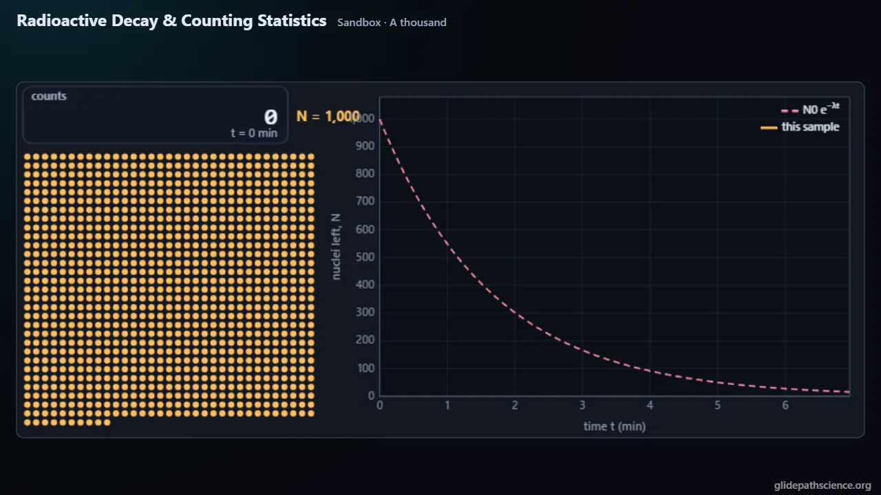
Every nucleus in this lab gets its own random lifetime, so one nucleus is unpredictable while a sample of thousands follows N = N₀e^(−λt), with T½ = ln 2/λ. A guided walkthrough at two levels reads a half-life from the curve, links λ to activity, and shows what a counter really counts: a fraction of the decays on top of a background, with a scatter of about √C that makes precision cost time. The Advanced track adds binomial survivors, waiting times, honest fits, dead time, detection limits and decay chains. The Sandbox runs up to 100,000 nuclei of any isotope on a counter of any efficiency, with charts of the nuclei left, counts per bin, count histograms and waiting times. A Counting Bench pools Geiger readings into a net rate with its uncertainty; a Dating Lab turns hours of counts into carbon-14 ages, or says a sample is too old to date; Decay Chains washes out a daughter and watches it grow back. A concept challenge and a prediction lab with fresh numbers on every run round it out.
What you'll learn
- Explain why no one can say when one nucleus will decay, yet half of a large sample decays in each half-life, following N = N₀e^(−λt) with T½ = ln 2/λ.
- Relate a counter’s rate to the activity, R = εA, and measure and subtract the background it sits on.
- Estimate a count’s uncertainty as about √C, and explain why counting four times as long halves the relative uncertainty.
- Fit a half-life from counts on a log plot, and date a sample from the carbon-14 left with an honest uncertainty, or say it is too old to date.
What you can do
- Guided walkthroughStep-by-step, in Intro and Advanced tracks.
- SandboxEvery control of the model, to explore freely.
- Virtual labA realistic experiment with measurement noise and data analysis.
- Concept checksQuestions about ideas and vocabulary, with no calculating.
- PredictionCommit to a prediction, then see the result.
- Classroom demoProjector mode and recordable clips for slides.
- Works offlineA single downloadable file, verified to run without a network.
Before you start
- Exponents, logarithms and graphs of exponential functions
- Atoms, nuclei and isotopes
- For the Advanced track: probability distributions (binomial and Poisson), variance, and least-squares fitting
Run or download
Run it in your browser
Nothing to install and no account. Works on laptops, Chromebooks, tablets, and phones.
Launch Radioactive Decay & Counting StatisticsDownload for offline use
One HTML file (719 kB) that opens in any modern browser with no network: for rooms with unreliable Wi-Fi, or to keep a copy.
Download the fileFile details and checksum
- File
radioactive-decay-counting-v1.1.html- Version
- 1.1, released November 15, 2026
- Build
f6de898- Size
- 735,970 bytes
- SHA-256
4887014ce93ed61dd19584d7a8b7edec0c40491f01dde15f1ec223c547c00455- Offline
- Checked to run with all network access blocked.
The model and its limits
What the model assumes
- Each of up to 100,000 nuclei gets its own random lifetime, t = −ln(u)/λ, from a seeded generator, so there is no time step, the survivors are exactly binomial, and a seed replays a run exactly.
- A counter catches each decay with probability ε; background arrives as an independent Poisson process; dead time drops clicks event by event, nonparalyzable or paralyzable.
- Half-lives are fit by Poisson maximum likelihood on the raw counts per bin with the background known; the Advanced comparison is a weighted least-squares fit of ln(net counts).
- Detection limits follow Currie’s critical level and detection limit; ages are quoted ± one standard deviation, or as lopsided intervals where the logarithm makes them so.
- Decay chains use Bateman’s closed form, with 2,000 nuclei followed through the chain; half-lives come from nuclear data tables (NUBASE2020 and NNDC).
What it leaves out
- No radiation physics: alpha, beta and gamma energies, ranges, shielding, absorbed dose and biological effects are left out.
- The detector’s energy response, plateau and geometry are folded into one efficiency; self-absorption in thick samples and random coincidences beyond dead time are not modeled.
- Radiocarbon ages come from the decay law alone, with today’s ratio assumed for the past; real laboratories correct with calibration curves.
- Every parent in a chain feeds the daughter (no branching ratios), and decay rates never change with chemistry.
Cite this simulation
APA 7
Meier, D. (2026). Radioactive Decay & Counting Statistics (Version 1.1) [Computer simulation]. Glidepath Science. https://glidepathscience.org/simulations/radioactive-decay-counting/
MLA 9
Meier, David. Radioactive Decay & Counting Statistics. Version 1.1, Glidepath Science, 2026, glidepathscience.org/simulations/radioactive-decay-counting/.
AIP
D. Meier, Radioactive Decay & Counting Statistics, version 1.1 (Glidepath Science, 2026), https://glidepathscience.org/simulations/radioactive-decay-counting/.
BibTeX
@misc{meier2026radioactivedecaycountingstatistics,
  author       = {Meier, David},
  title        = {{Radioactive Decay & Counting Statistics}},
  year         = {2026},
  publisher    = {Glidepath Science},
  version      = {1.1},
  note         = {Interactive simulation, version 1.1},
  howpublished = {\url{https://glidepathscience.org/simulations/radioactive-decay-counting/}},
  url          = {https://glidepathscience.org/simulations/radioactive-decay-counting/}
}
Credits and license
Created by Dr. David Meier, Glidepath Science.
Based on: OpenStax, University Physics Volume 3, by Samuel J. Ling, Jeff Sanny and William Moebs: The chapter “Nuclear Physics” (Chapter 10, §10.3 Radioactive Decay), an open textbook licensed CC BY-NC-SA 4.0 (openstax.org). The Intro track follows its order of topics and its notation for decay; the text, numbers, figures and simulations are this lab’s own. No endorsement by OpenStax or the authors is implied.
Licensed under Creative Commons Attribution-NonCommercial-ShareAlike 4.0 International (CC BY-NC-SA 4.0). You may share and adapt it for noncommercial purposes, such as teaching, with credit and under the same license. Licensing and reuse
AI tools (Claude, from Anthropic, and ChatGPT, from OpenAI) were used in developing Glidepath Science and its simulations. Dr. David Meier reviewed, edited, and modified every release version.