
NewVersion 1.1
Spectrophotometry & Beer’s Law
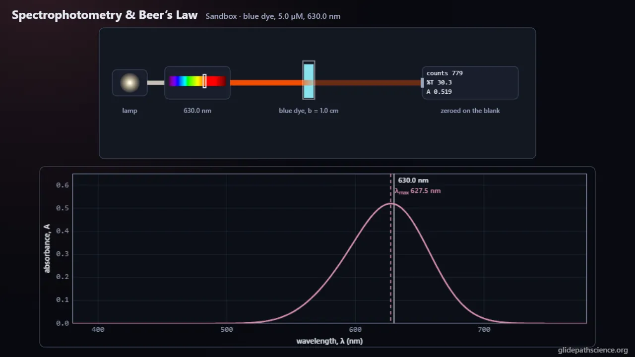
Shine one color of light through a dye, turn %T into absorbance, find λmax and watch A grow with concentration and path, then build a calibration line from standards and find an unknown.
About this simulation
Light falls by the same fraction in each slice of a solution, so transmittance falls exponentially while absorbance, A = −log₁₀ T, grows in a straight line. This lab makes that idea concrete with a single-beam spectrophotometer: a lamp, a monochromator, a cuvette and a detector that counts the light that gets through. A guided walkthrough at two levels covers %T and absorbance, zeroing on a blank, color and λmax, Beer’s law, A = εbc, standards, the calibration line, the unknown and the working range; the Advanced track adds Beer–Lambert from dI/dx, cross sections, mixtures read at two wavelengths, stray light and slit width, an isosbestic point, least squares, the unknown’s uncertainty, detection limits, the photometric error curve and standard addition. The Sandbox sets any dye, or a pH indicator, at any concentration, path and wavelength, scans spectra and plots A against c live. A Calibration Bench pipettes standards from a stock, measures each with honest noise, fits the line and reports an unknown. A concept challenge and a prediction lab with fresh numbers on every run round it out.
What you'll learn
- Explain why transmittance, T = I/I₀, falls exponentially through a solution while absorbance, A = −log₁₀ T, grows in a straight line.
- Use Beer’s law, A = εbc, to predict that doubling the concentration or the path doubles the absorbance, with ε the molecule’s own at one wavelength.
- Calibrate a measurement: zero on a blank, read at λmax, make standards by dilution, fit A against c, and read an unknown inside the standards’ range.
- Explain how stray light, a wide slit and equilibria bend the calibration line, how noise sets the detection limit, and why precision is best near A ≈ 0.4.
What you can do
- Guided walkthroughStep-by-step, in Intro and Advanced tracks.
- SandboxEvery control of the model, to explore freely.
- Virtual labA realistic experiment with measurement noise and data analysis.
- Concept checksQuestions about ideas and vocabulary, with no calculating.
- PredictionCommit to a prediction, then see the result.
- Classroom demoProjector mode and recordable clips for slides.
- Works offlineA single downloadable file, verified to run without a network.
Before you start
- Concentration in moles per liter and dilution
- Logarithms and straight-line graphs
- For the Advanced track: exponential decay from a rate equation, least-squares fitting and propagation of uncertainty
Run or download
Run it in your browser
Nothing to install and no account. Works on laptops, Chromebooks, tablets, and phones.
Launch Spectrophotometry & Beer’s LawDownload for offline use
One HTML file (633 kB) that opens in any modern browser with no network: for rooms with unreliable Wi-Fi, or to keep a copy.
Download the fileFile details and checksum
- File
spectrophotometry-beers-law-v1.1.html- Version
- 1.1, released November 15, 2026
- Build
fb771a2- Size
- 648,018 bytes
- SHA-256
7db2812be0c7a0fffcf6165f78f794e1c49d3e8a5aba3c6d667a2d29545ec83a- Offline
- Checked to run with all network access blocked.
The model and its limits
What the model assumes
- The dyes are synthetic: each absorption spectrum is a sum of Gaussian bands chosen to behave like food dyes; the pH indicator is illustrative, with a pKa of 7.10.
- The lamp is a 3100 K blackbody times a detector response that rises toward the red, so blue readings get fewer counts.
- The meter has 0.1 % stray light built in, so its readings fall below Beer’s law above A ≈ 1.5 and level off at A = 3.00; in Advanced the stray light runs from 0 to 5 %.
- An Advanced triangular slit averages T, not A, across its band; the Bench adds 0.15 %T of detector noise from a seeded generator, and the Sandbox’s readings are noiseless.
What it leaves out
- No scattering or fluorescence.
- No change of reflection with the solution’s refractive index, and no temperature effects.
- The bands’ quantum origin is not modeled, and the dyes’ spectra are not those of real compounds.
Cite this simulation
APA 7
Meier, D. (2026). Spectrophotometry & Beer’s Law (Version 1.1) [Computer simulation]. Glidepath Science. https://glidepathscience.org/simulations/spectrophotometry-beers-law/
MLA 9
Meier, David. Spectrophotometry & Beer’s Law. Version 1.1, Glidepath Science, 2026, glidepathscience.org/simulations/spectrophotometry-beers-law/.
AIP
D. Meier, Spectrophotometry & Beer’s Law, version 1.1 (Glidepath Science, 2026), https://glidepathscience.org/simulations/spectrophotometry-beers-law/.
BibTeX
@misc{meier2026spectrophotometrybeerslaw,
  author       = {Meier, David},
  title        = {{Spectrophotometry & Beer’s Law}},
  year         = {2026},
  publisher    = {Glidepath Science},
  version      = {1.1},
  note         = {Interactive simulation, version 1.1},
  howpublished = {\url{https://glidepathscience.org/simulations/spectrophotometry-beers-law/}},
  url          = {https://glidepathscience.org/simulations/spectrophotometry-beers-law/}
}
Credits and license
Created by Dr. David Meier, Glidepath Science.
Licensed under Creative Commons Attribution-NonCommercial-ShareAlike 4.0 International (CC BY-NC-SA 4.0). You may share and adapt it for noncommercial purposes, such as teaching, with credit and under the same license. Licensing and reuse
AI tools (Claude, from Anthropic, and ChatGPT, from OpenAI) were used in developing Glidepath Science and its simulations. Dr. David Meier reviewed, edited, and modified every release version.