
NewVersion 1.3
Potential Map
Map equipotentials on conductive paper with a virtual multimeter, compare them with point charges, find field-free hollows and sharp points, and see how ECG leads read the heart.
About this simulation
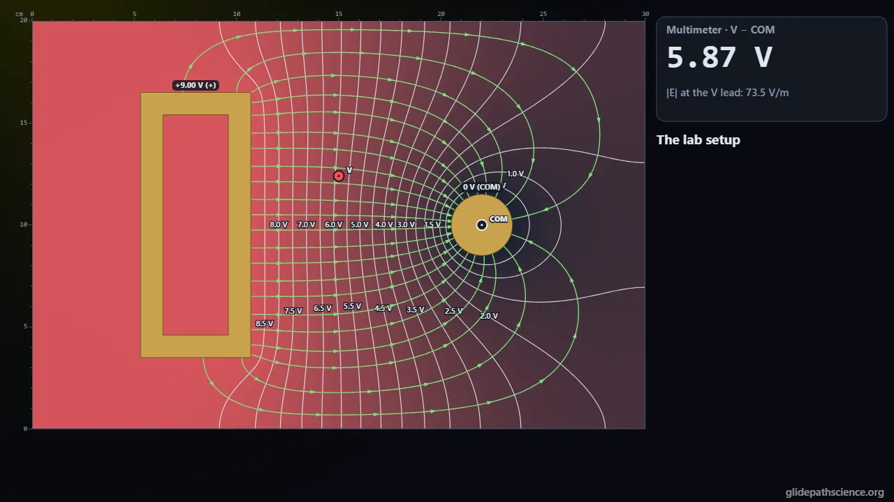
Electric potential as a map. Students survey a sheet of conductive paper with a two-lead multimeter, the way a surveyor maps a hillside: points at one voltage join into equipotentials, the field crosses them at right angles toward lower potential, and it is strongest where they crowd. The paper is solved for real (Laplace’s equation between brass electrodes held by a supply), with equal-flux field lines, field arrows to scale, a line scan, and a 3-D potential surface that turns; the same Sandbox places point charges in space, or line charges, so the two worlds can be compared. A Lab Bench gives black paper, brass electrodes, and a 3½-digit meter that rounds and scatters: chase an equipotential point by point, then reveal the true map and see how close you came, and in Advanced fit V against ln r and read the paper’s sheet resistance. A Heart & ECG tab models the heart as a moving current dipole in a 2-D torso, with the body-surface potential map through the beat, Einthoven’s triangle, and the six frontal leads on ECG paper. An Advanced track covers Laplace’s equation, the mean value and uniqueness, the 2-D world of the sheet, currents and capacitance, corners, floating conductors, cuts, images, the heart’s electrical axis, and lead fields.
What you'll learn
- Explain an equipotential as a set of points at one potential, why moving a charge along one takes no work, and why the field crosses it at right angles toward lower potential.
- Estimate the field from the spacing of equipotentials and from two meter readings, E ≈ −ΔV/Δs, and explain why a conductor is one equipotential with no field in a hollow.
- Compare conductive paper, where V solves Laplace’s equation and falls as −ln r, with point charges in space, where V adds as kq/r.
- Explain how an ECG lead reads the heart’s dipole projected on its own axis, why lead II = lead I + lead III, and find the electrical axis from the leads.
What you can do
- Guided walkthroughStep-by-step, in Intro and Advanced tracks.
- SandboxEvery control of the model, to explore freely.
- Virtual labA realistic experiment with measurement noise and data analysis.
- Concept checksQuestions about ideas and vocabulary, with no calculating.
- PredictionCommit to a prediction, then see the result.
- Classroom demoProjector mode and recordable clips for slides.
- Works offlineA single downloadable file, verified to run without a network.
Before you start
- Electric charge, force, and field at the level of Coulomb’s law
- Work and energy, and reading contour maps
- For the Advanced track: vector calculus (gradient, divergence) and Gauss’s law
Run or download
Run it in your browser
Nothing to install and no account. Works on laptops, Chromebooks, tablets, and phones.
Launch Potential MapDownload for offline use
One HTML file (986 kB) that opens in any modern browser with no network: for rooms with unreliable Wi-Fi, or to keep a copy.
Download the fileFile details and checksum
- File
potential-map-v1.3.html- Version
- 1.3, released November 15, 2026
- Build
387d18e- Size
- 1,009,699 bytes
- SHA-256
713cbb8771249ab1ddaa8dabfffad123d854fd66223480e2cdfb8c3719da849a- Offline
- Checked to run with all network access blocked.
The model and its limits
What the model assumes
- Conductive paper: a uniform 2-D sheet obeying Laplace’s equation, solved by finite volumes with electrodes cut at their true boundaries; insulating edges; electrodes are perfect conductors.
- Sheet resistance 5.0 kΩ per square for currents; potentials do not depend on it.
- Point charges in 3-D space and line charges, by exact superposition, with cores softened inside 2 mm.
- The bench meter: a 3½-digit DMM on its 20 V range with gain, offset, noise, and 0.5 mm placement scatter; seeded.
- The heart: a current dipole in a 2-D frontal-plane torso of uniform conductivity with insulated edges and current-free limb stubs; amplitudes calibrated to a normal lead II, not predicted.
What it leaves out
- The sheet is a 2-D world: its −ln r is not the 1/r of space.
- No paper thickness, anisotropy, temperature, corona, or breakdown at sharp points.
- The torso is a 2-D slice of a 3-D, inhomogeneous body; no chest leads (V1–V6), multipoles, electrode impedance, or filters.
- Non-uniform paper and a poorly pressed electrode on the bench are illustrative.
Cite this simulation
APA 7
Meier, D. (2026). Potential Map (Version 1.3) [Computer simulation]. Glidepath Science. https://glidepathscience.org/simulations/potential-map/
MLA 9
Meier, David. Potential Map. Version 1.3, Glidepath Science, 2026, glidepathscience.org/simulations/potential-map/.
AIP
D. Meier, Potential Map, version 1.3 (Glidepath Science, 2026), https://glidepathscience.org/simulations/potential-map/.
BibTeX
@misc{meier2026potentialmap,
  author       = {Meier, David},
  title        = {{Potential Map}},
  year         = {2026},
  publisher    = {Glidepath Science},
  version      = {1.3},
  note         = {Interactive simulation, version 1.3},
  howpublished = {\url{https://glidepathscience.org/simulations/potential-map/}},
  url          = {https://glidepathscience.org/simulations/potential-map/}
}
Credits and license
Created by Dr. David Meier, Glidepath Science.
Licensed under Creative Commons Attribution-NonCommercial-ShareAlike 4.0 International (CC BY-NC-SA 4.0). You may share and adapt it for noncommercial purposes, such as teaching, with credit and under the same license. Licensing and reuse
AI tools (Claude, from Anthropic, and ChatGPT, from OpenAI) were used in developing Glidepath Science and its simulations. Dr. David Meier reviewed, edited, and modified every release version.