
NewVersion 1.3
Parallel Plates & Uniform Fields
Charge two plates and explore the uniform field between them: work and potential energy in electronvolts, beams fired onto a screen, fringe fields, and Millikan’s oil drops counted in whole electrons.
About this simulation
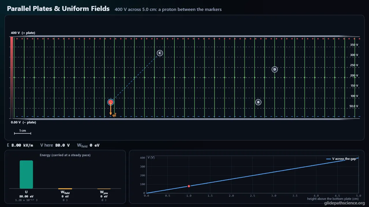
Two charged plates make the simplest field there is: the same push everywhere in the gap. Students carry charges between markers by any route and watch a work meter add up qE·Δs piece by piece, release and launch protons, electrons, and ions, and fire beams through the gap onto a screen, all in exact closed-form motion with energy bars in electronvolts and joules. An Advanced track adds Laplace’s equation and surface charge, fringe fields from a boundary-element field engine and the loop argument for why they must exist, sparks at the edges, one path for every ion from one gun, the exact relativistic deflection, Child’s space-charge law, and Millikan’s experiment measured properly with Stokes drag, slip, and Brownian motion. A Deflection Lab measures a tube’s sensitivity from noisy spot readings and turns into an oscilloscope with sweeps and Lissajous figures; a Millikan Bench lets students time their own oil drops, ionize them, and find e.
What you'll learn
- Use E = ΔV/d for the uniform field between parallel plates, the same in strength and direction everywhere in the gap, with equipotentials parallel to the plates.
- Find the change in potential energy, ΔU = qΔV, and the field’s work, −qΔV, for positive and negative charges by any route, in joules and electronvolts.
- Predict the parabolic path of a charge fired between the plates and the spot on a screen, and explain why ions from one gun share one path.
- Find a drop’s charge from a balance voltage or from timed fall and rise speeds, and show that every charge is a whole number of e.
What you can do
- Guided walkthroughStep-by-step, in Intro and Advanced tracks.
- SandboxEvery control of the model, to explore freely.
- Virtual labA realistic experiment with measurement noise and data analysis.
- Concept checksQuestions about ideas and vocabulary, with no calculating.
- PredictionCommit to a prediction, then see the result.
- Classroom demoProjector mode and recordable clips for slides.
- Works offlineA single downloadable file, verified to run without a network.
Before you start
- Electric field and electric potential, and F = qE
- Kinetic energy and constant-acceleration (projectile) motion
- For the Advanced track: calculus, Gauss’s law, and an introduction to special relativity
Run or download
Run it in your browser
Nothing to install and no account. Works on laptops, Chromebooks, tablets, and phones.
Launch Parallel Plates & Uniform FieldsDownload for offline use
One HTML file (1.0 MB) that opens in any modern browser with no network: for rooms with unreliable Wi-Fi, or to keep a copy.
Download the fileFile details and checksum
- File
parallel-plates-v1.3.html- Version
- 1.3, released November 15, 2026
- Build
23cc35a- Size
- 1,055,343 bytes
- SHA-256
1ab81395176f51f3ddb556012546a259bdb38c46f8365a2616b5469954114c3f- Offline
- Checked to run with all network access blocked.
The model and its limits
What the model assumes
- Ideal plates by default: a uniform field between them and none outside, so motion is the exact constant-acceleration solution with plate hits found as polynomial roots.
- Finite plates (Advanced) are two-dimensional, long into the page, solved by boundary elements with one stored solution per plate; motion through them is integrated adaptively, with K + qV conserved to about one part in a million.
- Relativistic beams follow the exact solution for a constant transverse field: p_x constant, p_y = qEt.
- Space charge appears only as the analytic Child–Langmuir gap.
- Oil drops move at terminal speed (their relaxation time is microseconds), with Stokes drag reduced by the linear Cunningham slip factor, Sutherland’s air viscosity, buoyancy, and seeded Brownian steps.
- The Deflection Lab’s spot is the engine’s deflection plus a seeded jitter and, in Realistic mode, a stray-field zero offset.
What it leaves out
- Finite plates are two-dimensional, so their fringe field reaches farther than real plates’ would.
- No magnetic fields except the Deflection Lab’s zero offset (magnetic deflection is in Force on a Moving Charge).
- No supply resistance or charging transients, no dielectrics, no radiation, and no gravity for ions and electrons.
- Relativity is left out of the Intro track and of released charges.
- The slip correction uses the linear Cunningham form, valid while b/(pr) is below about 0.3; drops do not evaporate and the chamber has no convection.
- Millikan’s historical data and the history of his drop selection are given as published accounts, to be verified.
Cite this simulation
APA 7
Meier, D. (2026). Parallel Plates & Uniform Fields (Version 1.3) [Computer simulation]. Glidepath Science. https://glidepathscience.org/simulations/parallel-plates/
MLA 9
Meier, David. Parallel Plates & Uniform Fields. Version 1.3, Glidepath Science, 2026, glidepathscience.org/simulations/parallel-plates/.
AIP
D. Meier, Parallel Plates & Uniform Fields, version 1.3 (Glidepath Science, 2026), https://glidepathscience.org/simulations/parallel-plates/.
BibTeX
@misc{meier2026parallelplatesuniformfields,
  author       = {Meier, David},
  title        = {{Parallel Plates & Uniform Fields}},
  year         = {2026},
  publisher    = {Glidepath Science},
  version      = {1.3},
  note         = {Interactive simulation, version 1.3},
  howpublished = {\url{https://glidepathscience.org/simulations/parallel-plates/}},
  url          = {https://glidepathscience.org/simulations/parallel-plates/}
}
Credits and license
Created by Dr. David Meier, Glidepath Science.
Licensed under Creative Commons Attribution-NonCommercial-ShareAlike 4.0 International (CC BY-NC-SA 4.0). You may share and adapt it for noncommercial purposes, such as teaching, with credit and under the same license. Licensing and reuse
AI tools (Claude, from Anthropic, and ChatGPT, from OpenAI) were used in developing Glidepath Science and its simulations. Dr. David Meier reviewed, edited, and modified every release version.