
NewVersion 1.1
Magnetic Fields from Currents
Map the field around wires, loops and solenoids with compasses and a probe, build Biot–Savart piece by piece, test Ampère’s law on paths you draw, and find the force between currents.
About this simulation
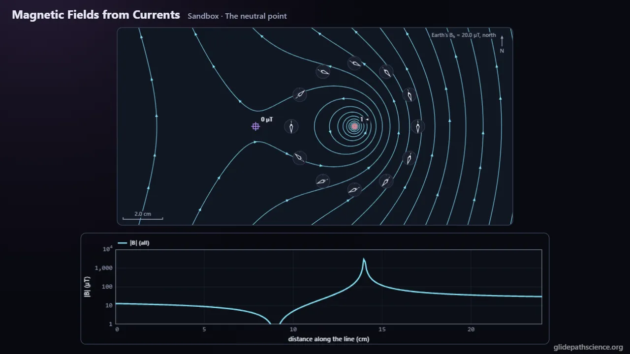
Where does a current’s magnetic field point, and how strong is it? Students run wires, a coaxial cable, a strip or a toroid through a tabletop seen from above, with Earth’s field and compasses that swing like real needles, and read the field lines, a map of |B| and the forces between wires; a second view shows coils and a solenoid from the side. A guided walkthrough at two levels runs from a compass beside a current through Biot–Savart, the long wire, the force between currents and a loop’s axis to Ampère’s law, the thick wire and the toroid; the Advanced track adds polygons, the dipole far field, the Helmholtz pair, winding numbers, the coax, the curl, an iron core and Maxwell’s displacement current. A Biot–Savart Builder adds up a shape’s field one piece at a time, an Ampère Loop Lab sets ∮B·dl beside μ₀ times the enclosed current for any path drawn, and a Field Bench measures Earth’s field and μ₀ with honest instruments. Concept challenges and a prediction lab with fresh numbers round it out.
What you'll learn
- Build a current’s field from Biot–Savart, dB = (μ₀/4π) I dl sin θ/r², and sum it to μ₀I/2πR for a long wire and μ₀NI/2R at the center of a loop.
- Read the field with a compass, which shows the net horizontal field of Earth and the current together, and with a probe, which reads one component, Earth’s included unless it is zeroed.
- Find the force per length between parallel currents, F/l = μ₀I₁I₂/2πr, attracting when they run the same way, and explain why the two forces are equal and opposite however unequal the currents.
- Apply Ampère’s law, ∮B·dl = μ₀I_enc, around any path, and use symmetry to find B inside a thick wire, a coaxial cable, a toroid and a solenoid.
What you can do
- Guided walkthroughStep-by-step, in Intro and Advanced tracks.
- SandboxEvery control of the model, to explore freely.
- Virtual labA realistic experiment with measurement noise and data analysis.
- Concept checksQuestions about ideas and vocabulary, with no calculating.
- PredictionCommit to a prediction, then see the result.
- Classroom demoProjector mode and recordable clips for slides.
- Works offlineA single downloadable file, verified to run without a network.
Before you start
- Vectors, the cross product and the right-hand rule
- Current and the magnetic force on a moving charge (Force on a Moving Charge)
- For the Advanced track: line integrals, polar coordinates, and integrals of trigonometric functions
Run or download
Run it in your browser
Nothing to install and no account. Works on laptops, Chromebooks, tablets, and phones.
Launch Magnetic Fields from CurrentsDownload for offline use
One HTML file (883 kB) that opens in any modern browser with no network: for rooms with unreliable Wi-Fi, or to keep a copy.
Download the fileFile details and checksum
- File
magnetic-fields-from-currents-v1.1.html- Version
- 1.1, released November 15, 2026
- Build
556fae1- Size
- 904,298 bytes
- SHA-256
756846f5c23806ef1385b955e2a261713595fcfd6193c39e6da0ca89f565c96f- Offline
- Checked to run with all network access blocked.
The model and its limits
What the model assumes
- Magnetostatics: steady currents and exact superposition, with μ₀ from CODATA 2022; long wires, exact finite segments, loops by elliptic integrals and solenoids as current sheets.
- Ampère’s law is shown twice: ∮B·dl is integrated numerically along the drawn path, and the enclosed current is counted separately by winding numbers.
- Earth’s field is uniform, 20.0 µT north and inclined 65°, an illustrative mid-latitude value.
- The compass is a 2.0 cm steel needle with its own magnetic moment, damping and pivot friction, so it swings and settles like a real one.
- The Advanced iron core appears only in a closed toroid: linear with a relative permeability of 2,000 up to 1.5 T, with no hysteresis.
What it leaves out
- Thin wires are lines, whose field grows without limit close to them; every source on the table is infinitely long, and a finite wire appears only in the Builder.
- Nothing changes in time: induction, self-inductance, AC and radiation are left out, and switching a current changes the field at once.
- No magnetic materials other than Earth’s field, the needle and the toroid’s linear core, and Earth’s field does not vary with place or time.
- A real winding’s one turn around the axis, the skin effect, the wires’ heating and their motion under the forces are left out.
Cite this simulation
APA 7
Meier, D. (2026). Magnetic Fields from Currents (Version 1.1) [Computer simulation]. Glidepath Science. https://glidepathscience.org/simulations/magnetic-fields-from-currents/
MLA 9
Meier, David. Magnetic Fields from Currents. Version 1.1, Glidepath Science, 2026, glidepathscience.org/simulations/magnetic-fields-from-currents/.
AIP
D. Meier, Magnetic Fields from Currents, version 1.1 (Glidepath Science, 2026), https://glidepathscience.org/simulations/magnetic-fields-from-currents/.
BibTeX
@misc{meier2026magneticfieldsfromcurrents,
  author       = {Meier, David},
  title        = {{Magnetic Fields from Currents}},
  year         = {2026},
  publisher    = {Glidepath Science},
  version      = {1.1},
  note         = {Interactive simulation, version 1.1},
  howpublished = {\url{https://glidepathscience.org/simulations/magnetic-fields-from-currents/}},
  url          = {https://glidepathscience.org/simulations/magnetic-fields-from-currents/}
}
Credits and license
Created by Dr. David Meier, Glidepath Science.
Based on: OpenStax, University Physics Volume 2, by Samuel J. Ling, Jeff Sanny and William Moebs: Chapter 12, “Sources of Magnetic Fields,” §12.1–12.7, with §11.2 for compasses and field lines, an open textbook licensed CC BY-NC-SA 4.0 (openstax.org). The order of topics and the notation follow it; the text, numbers, figures and simulations are this lab’s own. No endorsement by the authors or OpenStax is implied.
Licensed under Creative Commons Attribution-NonCommercial-ShareAlike 4.0 International (CC BY-NC-SA 4.0). You may share and adapt it for noncommercial purposes, such as teaching, with credit and under the same license. Licensing and reuse
AI tools (Claude, from Anthropic, and ChatGPT, from OpenAI) were used in developing Glidepath Science and its simulations. Dr. David Meier reviewed, edited, and modified every release version.