
NewVersion 1.4
Flux Counter
Count field lines through a closed surface you drag, then turn the count into Gauss’s law: flux, enclosed charge, and the fields of spheres, lines, sheets, and conductors.
About this simulation
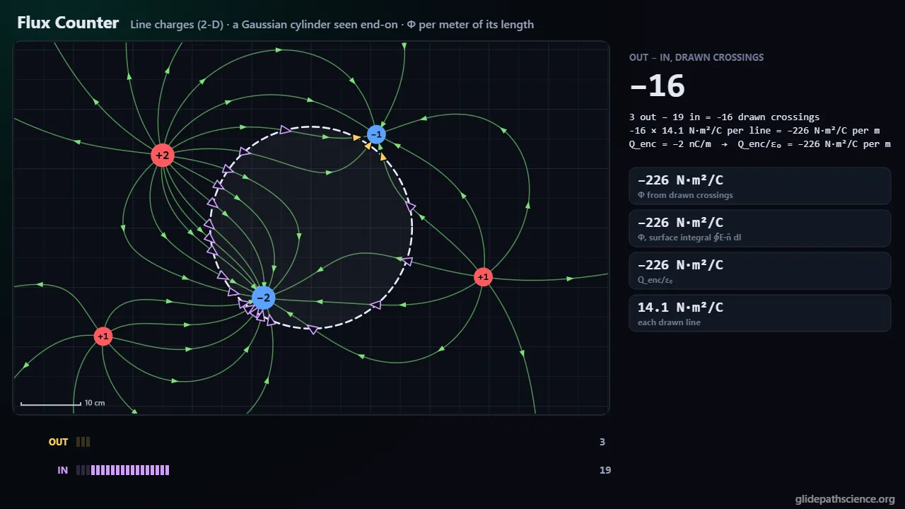
Drag a Gaussian surface across charged rods and tally every field line that crosses it, out and in: the net depends only on the charge inside, never on the surface’s shape or the charges outside. Flux is computed independently by integrating E over the surface, for line charges in 2-D, point charges in 3-D, and a flat patch in a uniform field. A Symmetry Lab turns Gauss’s law into E for a point charge, a shell, a ball, a line, a cylinder, a sheet, and a conductor with a cavity, and shows why it cannot for a finite rod. The Advanced track adds solid angle, charges on the boundary, the divergence, where flat line drawings stop telling the truth, and Gauss’s law for gravity.
What you'll learn
- Count the charge: out minus in counts the charge inside, at 8 lines for every nC/m as the board usually draws them, and lines from charges outside enter and leave again.
- Only the inside counts: the surface’s shape and size, and the charges outside it, never change the flux through a closed surface; only moving charge across it does.
- Φ = Q_enc/ε₀: each nC inside gives 113 N·m²/C of flux through any closed surface around it, and a flat patch in a uniform field gets EA cos θ.
- Symmetry gives E: when E is the same all over a sphere, cylinder, or pillbox, the flux is E times the area, and Gauss’s law gives E outright.
What you can do
- Guided walkthroughStep-by-step, in Intro and Advanced tracks.
- SandboxEvery control of the model, to explore freely.
- Concept checksQuestions about ideas and vocabulary, with no calculating.
- PredictionCommit to a prediction, then see the result.
- Classroom demoProjector mode and recordable clips for slides.
- Works offlineA single downloadable file, verified to run without a network.
Before you start
- Electric fields and Coulomb’s law
- Vectors and the dot product
- Areas of spheres and cylinders
- Surface integrals, for the Advanced track
Run or download
Run it in your browser
Nothing to install and no account. Works on laptops, Chromebooks, tablets, and phones.
Launch Flux CounterDownload for offline use
One HTML file (783 kB) that opens in any modern browser with no network: for rooms with unreliable Wi-Fi, or to keep a copy.
Download the fileFile details and checksum
- File
flux-counter-v1.4.html- Version
- 1.4, released November 15, 2026
- Build
a01a111- Size
- 801,983 bytes
- SHA-256
73ac27cb65d77453239931c50bb63110e2ecb30e5b646139fcce894da31d9ad4- Offline
- Checked to run with all network access blocked.
The model and its limits
What the model assumes
- In 2-D each charge is a long straight rod with E = λ/(2πε₀r), and every flux is per meter of the Gaussian cylinder’s length; in 3-D each charge is a point charge in the page with E = q/(4πε₀r²).
- Field lines are traced with fourth-order Runge–Kutta, and in 2-D a balancer re-aims lines so that every charge holds exactly n lines per nC/m; that is a drawing construction, not evidence for Gauss’s law.
- The crossing tally is pure topology: it counts where each line passes into or out of the surface and never looks at the field strength.
- Flux is also computed independently by integrating E over the surface: numerically around the curve in 2-D, over the whole sphere or by exact solid angles for the cube in 3-D.
- The Symmetry Lab’s closed forms are checked against Coulomb’s law integrated directly over each charge, which agree to better than a part in ten million off the charged surfaces.
What it leaves out
- Charges are fixed in place and lie in the page plane; nothing feels a force or moves.
- Conductors appear only in the Symmetry Lab, where their charges follow from Gauss’s law; there are no dielectrics and no fields that change in time.
- Field lines are a finite sample, charge cores are softened inside 2 mm, and lines are followed to 0.9 m beyond the board before they count as escaping to infinity.
- Infinite rods, lines, and sheets are idealizations, and an ideal charged surface has no single field value on it.
- In 3-D the count of lines drawn in the page is not a flux; the flux shown is always the integral over the whole sphere or cube.
Cite this simulation
APA 7
Meier, D. (2026). Flux Counter (Version 1.4) [Computer simulation]. Glidepath Science. https://glidepathscience.org/simulations/flux-counter/
MLA 9
Meier, David. Flux Counter. Version 1.4, Glidepath Science, 2026, glidepathscience.org/simulations/flux-counter/.
AIP
D. Meier, Flux Counter, version 1.4 (Glidepath Science, 2026), https://glidepathscience.org/simulations/flux-counter/.
BibTeX
@misc{meier2026fluxcounter,
  author       = {Meier, David},
  title        = {{Flux Counter}},
  year         = {2026},
  publisher    = {Glidepath Science},
  version      = {1.4},
  note         = {Interactive simulation, version 1.4},
  howpublished = {\url{https://glidepathscience.org/simulations/flux-counter/}},
  url          = {https://glidepathscience.org/simulations/flux-counter/}
}
Credits and license
Created by Dr. David Meier, Glidepath Science.
Licensed under Creative Commons Attribution-NonCommercial-ShareAlike 4.0 International (CC BY-NC-SA 4.0). You may share and adapt it for noncommercial purposes, such as teaching, with credit and under the same license. Licensing and reuse
AI tools (Claude, from Anthropic, and ChatGPT, from OpenAI) were used in developing Glidepath Science and its simulations. Dr. David Meier reviewed, edited, and modified every release version.